Deep Deterministic Policy Gradient - Another Improvement in solving Continuous Action Spaces

Introduction

A number of algorithms have been developed in the field of deep reinforcement learning - e.g. DQN, DDQN, Actor-Critic, and many others. They all have one thing in common: they are suitable (to varying degrees) for solving tasks with discrete action spaces. This is useful for relatively simple decision processes, but not sufficient for machine control tasks. To solve such a task, for example, the Deep Deterministic Policy Gradients algorithm was developed, which is able to deal efficiently with continuous action spaces.

This algorithm will be abbreviated as DDPG.

In this article, we will introduce the algorithm and discuss its strengths and weaknesses. Using an implementation, we will then demonstrate why this algorithm has become a cornerstone of current research and application in deep reinforcement learning.

Types of Action Spaces: Discrete vs Continuous

In our introduction to reinforcement learning and the Deep Q-Network (DQN) algorithm, we implicitely showed the importance of the action space in defining how an agent interacts with its environment. Initially, we only focused on discrete action spaces, where the set of possible actions is composed of a finite number of distinct states.

Discrete Action Spaces

In discrete action spaces, the action space consists of a countable infinity of possible actions. The choice between these actions is based on a probability distribution over the available actions. ¹ For instance:

• In the classic game of Pac-Man, the player can choose to move up, down, left, or right, with each action having a corresponding reward structure.
• A robot navigating through a grid can take only four possible actions at any given state: up, down, left, or right.

These examples illustrate the limitations of discrete action spaces. In certain scenarios, the agent may need to make non-binary decisions that cannot be represented by a simple probability distribution over distinct states.

Continuous Action Spaces

In contrast, continuous action spaces offer a more nuanced and detailed representation of the environment. The action space consists of a range of values rather than distinct states, allowing the agent to take any value within this range based on its sensory inputs. ²

• A robotic arm in a warehouse environment can move its end effector to any position within a 3D cube, with the arm’s position and velocity being continuous quantities.
• In a driving scenario, the car’s acceleration is continuous, enabling smooth acceleration and deceleration.

Continuous action spaces provide a more realistic representation of many real-world environments, where actions can take on any value within a range. This distinction between discrete and continuous action spaces is crucial in reinforcement learning, as it influences the choice of algorithms and models used to solve complex problems.

For continuous action spaces, the range of values can either be limited by an upper and/or lower bound or entirely unlimited. The underlying problem that should be modeled in an environment has to provide the corresponding limitations.

Realistic action spaces, that consist of more than a single dimension, might be comprised of both (limited/unlimited) continuous dimensions and discrete dimensions.

Technical Background

The Deep Deterministic Policy Gradient (DDPG) algorithm is a model-free reinforcement learning algorithm that uses a combination of policy gradients and value functions to learn optimal policies in complex, continuous environments. In short, it is based on the actor critic algorithm.

The main change that is made in the basic algorithm from actor critic to ddpg is the fact that we utilize a deterministic policy over a stochastic policy to sample our action. In order to maintain our exploration during training, we utilize a random noise, which we can specify.

Algorithm

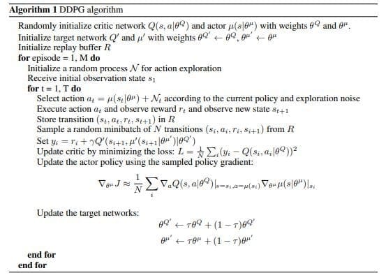
Now, we present the pseudocode for implementing the DDPG algorithm. This pseudocode extends the basic idea of DDPG with the usage of target networks for both the actor and the critic, in order to slow down parameter changes. This attempt is implemented to avoid overshooting during training.

If you want to learn more about the usage of target networks in reinforcement learning, you can visit the DDQN page.

Implementation

We now present an implementation for DDPG, which is based on the pseudocode above. Some of our code is based upon this tutorial from keras, like the random noise generation we utilized here.

For our implementation, we begin with our imports and supportive functionalities.

Please note: Since our last reinforcement learning code article, OpenAI Gym has been renamed to OpenAI Gymnasium. Therefore, we import gymnasium instead of gym.

import numpy as np
import pandas as pd
import tensorflow as tf

import gymnasium as gym

from tensorflow.python.keras import Model
from tensorflow.python.keras.optimizer_v2.adam import Adam
from tensorflow.python.keras.layers import Input, Dense, Concatenate

def avg_n(list1, n = 50):
    if (len(list1) > n):
        return np.average(list1[len(list1) - n:len(list1)])
    else:
        return np.average(list1[0:len(list1)])

Now, we implement our random noise, necessary to generate an exploration path for our agent. For this, we utilize the Ornstein-Uhlenbeck process, a process for sampling random noise in an efficient manner. It is so effective, because we can numerically approximate the next random number with a simple formula, given the last random number and a variety of parameters.

class OUActionNoise:
    def __init__(self, mean, std_deviation, theta=0.15, dt=1e-2, x_initial=None):
        self.theta = theta
        self.mean = mean
        self.std_dev = std_deviation
        self.dt = dt
        self.x_initial = x_initial
        self.reset()

    def __call__(self):
        x = (self.x_prev + self.theta * (self.mean - self.x_prev) * self.dt + self.std_dev * np.sqrt(self.dt) * np.random.normal(size=self.mean.shape))
        self.x_prev = x
        return x

    def reset(self):
        if self.x_initial is not None:
            self.x_prev = self.x_initial
        else:
            self.x_prev = np.zeros_like(self.mean)

Nextup, we implement an experience memory identical to the DQN experience replay.

class ExperienceMemory:
    def __init__(self, observation_size, action_size, memory_capacity=100000, batch_size=64):
        self.memory_capacity = memory_capacity
        self.batch_size = batch_size
        self.clength = 0

        self.cstate_memory = np.zeros((self.memory_capacity, observation_size))
        self.action_memory = np.zeros((self.memory_capacity, action_size))
        self.reward_memory = np.zeros((self.memory_capacity, 1))
        self.pstate_memory = np.zeros((self.memory_capacity, observation_size))

    def record(self, cstate, action, reward, pstate):
        # Set index to zero if buffer_capacity is exceeded, replacing old records
        index = self.clength % self.memory_capacity 

        self.cstate_memory[index] = cstate
        self.action_memory[index] = action
        self.reward_memory[index] = reward
        self.pstate_memory[index] = pstate

        self.clength += 1

    def sample_batches(self):
        # Sampling indices from the experience memory
        record_range = min(self.clength, self.memory_capacity)
        batch_indices = np.random.choice(record_range, self.batch_size)

        # Convert to tensors
        state_batch = tf.convert_to_tensor(self.cstate_memory[batch_indices])
        action_batch = tf.convert_to_tensor(self.action_memory[batch_indices])
        reward_batch = tf.convert_to_tensor(self.reward_memory[batch_indices])
        reward_batch = tf.cast(reward_batch, dtype=tf.float32)
        next_state_batch = tf.convert_to_tensor(self.pstate_memory[batch_indices])

        return (state_batch, action_batch, reward_batch, next_state_batch)

Afterwards, we implement our soft update function, that accepts the weigts of any neural network. We will use it later for both of our target networks.

@tf.function
def update_target(target_weights, weights, tau: float):
    for (target_weight, primary_weight) in zip(target_weights, weights):
        target_weight.assign(primary_weight * tau + target_weight * (1 - tau))

As a next step, we begin the implementation of our DDPG agent class. Here, we have a variety of functions, which serve different purposes:

1. __init__: Initializes all hyperparameters, random noise instances, experience replay, and neural networks.
2. build_actor: Constructs the architecture and weights for the actor networks. Notably, the target network is initialized by copying the weights of the first network.

The actor network leverages a tf.random_uniform_initializer to enhance convergence.

3. build_critic: Establishes the architecture and weights for the critic networks. Unlike traditional models, the critic network utilizes both state and action inputs to predict the quality of the next action. This approach allows for a more comprehensive understanding of the environment.

A crucial aspect of the critic model is its implementation using the Functional API of TensorFlow. While the Sequential API can be used for actor implementations, we chose to employ the Functional API consistently to maintain coherence. The parallel processing inherent in this approach enables us to effectively combine state and action information before making predictions.

class DDPGAgent:
    def __init__(self, observation_size, action_size, lower_bound, upper_bound):
        self.observation_size = observation_size
        self.action_size = action_size
        self.lower_bound = lower_bound
        self.upper_bound = upper_bound

        self.standard_deviation = 0.2
        self.ou_noise = OUActionNoise(mean=np.zeros(1), std_deviation=float(self.standard_deviation) * np.ones(1))

        # Initialize primary and target networks
        self.actor_model = self.build_actor()
        self.critic_model = self.build_critic()
        self.target_actor = self.build_actor()
        self.target_critic = self.build_critic()

        # Creating equal weights for both primary and target networks
        self.target_actor.set_weights(self.actor_model.get_weights())
        self.target_critic.set_weights(self.critic_model.get_weights())

        # Initialize network parameters
        self.alpha1 = 1e-5
        self.alpha2 = 1e-3
        self.memory_length = 10000
        self.batch_size = 64
        self.gamma = 0.99
        self.tau = 0.005

        # Initalize the Experience Memory
        self.memory = ExperienceMemory(observation_size=observation_size, action_size=action_size)

        # Initialize the optimizers
        self.actor_optimizer = Adam(self.alpha1)
        self.critic_optimizer = Adam(self.alpha2)

    def build_actor(self):
        last_init = tf.random_uniform_initializer(minval=-0.003, maxval=0.003) # Initialize weights between -3e-3 and 3-e3

        inputs = Input(shape=(self.observation_size,))
        out = Dense(128, activation="relu")(inputs)
        out = Dense(64, activation="relu")(out)
        outputs = Dense(self.action_size, activation="tanh", kernel_initializer=last_init)(out)

        outputs = outputs * self.upper_bound
        model = Model(inputs, outputs)
        
        return model

    def build_critic(self):
        state_input = Input(shape=self.observation_size)
        state_out = Dense(32, activation="relu")(state_input)

        action_input = Input(shape=(self.action_size))
        action_out = Dense(64, activation="relu")(action_input)

        concat = Concatenate()([state_out, action_out])

        out = Dense(256, activation="relu")(concat)
        out = Dense(128, activation="relu")(out)
        outputs = Dense(1)(out)

        model = Model([state_input, action_input], outputs)

        return model

      def store_episode(self, cstate, action, reward, pstate):
        self.memory.record(cstate, action, reward, pstate)

Next, we implement the policy function, building upon the established pattern from our previous actor-critic algorithm implementation. The key difference lies in the clipping of the sampled action, ensuring that it falls within the defined action boundaries of our environment.

    def policy(self, state):
        state = tf.expand_dims(state, axis=0)
        sampled_actions = tf.squeeze(self.actor_model(state))
        
        noise = self.ou_noise()
        sampled_actions = sampled_actions.numpy() + noise

        # Clip sampled action to our bounds, making sure it is not out of bounds.
        legal_action = np.clip(sampled_actions, self.lower_bound, self.upper_bound)

        return [np.squeeze(legal_action)]

Following the implementation of the policy function, we move on to the update method. For this step, we apply the update formulas derived from the pseudocode and incorporate the updated weights for both the actor and critic networks.

We also utilize the @tf.function decorator to optimize execution speed. By leveraging TensorFlow’s internal graph-building capabilities, this annotation enables significant performance improvements. The method is converted into a callable TensorFlow graph, which facilitates efficient backtracing of prediction errors during training.

    @tf.function
    def update(self, state_batch, action_batch, reward_batch, next_state_batch):
        # Applying gradients for the critic model
        with tf.GradientTape() as tape:
            target_actions = self.target_actor(next_state_batch, training=True)
            y = reward_batch + self.gamma * self.target_critic([next_state_batch, target_actions], training=True)
            critic_value = self.critic_model([state_batch, action_batch], training=True)
            critic_loss = tf.math.reduce_mean(tf.math.square(y - critic_value)) # MSE

        critic_grad = tape.gradient(critic_loss, self.critic_model.trainable_variables)
        self.critic_optimizer.apply_gradients(zip(critic_grad, self.critic_model.trainable_variables))

        # Applying gradients for the actor model
        with tf.GradientTape() as tape:
            actions = self.actor_model(state_batch, training=True)
            critic_value = self.critic_model([state_batch, actions], training=True)
            actor_loss = -tf.math.reduce_mean(critic_value)

        actor_grad = tape.gradient(actor_loss, self.actor_model.trainable_variables)
        self.actor_optimizer.apply_gradients(zip(actor_grad, self.actor_model.trainable_variables))

In the final step before completing our agent implementation, we examine the train method. This method serves as a streamlined solution for training, combining the updates from both the actor and critic networks, along with soft updates. To simplify this process, we opted to implement it as a single, self-contained method.

However, there’s an important consideration when it comes to sampling experiences from our experience memory. Due to its inherent non-determinism, this process cannot be seamlessly integrated into a callable graph, which would enable the use of TensorFlow’s @tf.function decorator. As a result, we’ve chosen to implement the train method in a way that allows for efficient training while still respecting these limitations.

    def train(self):
        cstates, actions, rewards, pstates = self.memory.sample_batches()

        # Updating the main networks
        self.update(cstates, actions, rewards, pstates)

        # Executing soft updates for the target networks
        update_target(self.target_critic.variables, self.critic_model.variables, self.tau)
        update_target(self.target_actor.variables, self.actor_model.variables, self.tau)

As a final step, we provide you with any external code snippets, necessary to train your model on the Ant-v5 environment of the OpenAI gymnasium.

def training_loop(env, agent: DDPGAgent, max_frames_episode):
  current_obs, _ = env.reset()
  episode_reward = 0

  for j in range(max_frames_episode):
    action = agent.policy(current_obs)

    next_obs, reward, done, _, _ = env.step(action)
    next_obs = np.array(next_obs)

    # Store all episode information for training process
    agent.store_episode(current_obs, action, reward, next_obs)

    # Reseting environment information so that next episode can handle the previous information
    current_obs = next_obs
    episode_reward += reward

    if done:
      break

  return episode_reward, agent

n_episodes, max_frames_episode, current_episode, avg_length, evaluation_interval = 500, 500, 0, 50, 10
episodic_reward, avg_reward, eps_value, evaluation_rewards = [], [], [], []

# env = gym.make("LunarLander-v2", continuous=True, gravity = -10.0, enable_wind=False, wind_power=15.0, turbulence_power=1.5)
env = gym.make('MountainCarContinuous-v0')

seed = 69
tf.random.set_seed(seed)
np.random.seed(seed)

n_actions, observation_shape = env.action_space.shape[0], env.observation_space.shape[0]
lower_bound, upper_bound = env.action_space.low[0], env.action_space.high[0]

agent = DDPGAgent(observation_shape, n_actions, lower_bound, upper_bound)

for i in range(n_episodes):
    current_episode += 1
    episode_reward, agent = training_loop(env, agent, max_frames_episode)
        
    if (current_episode % 20 == 0):
        print("Episode {} - ".format(current_episode), "Episodic Reward: {}".format(episode_reward))
        
    episodic_reward.append(episode_reward)
    current_average = avg_n(episodic_reward, n=avg_length)
    avg_reward.append(current_average)
    agent.train()
            
    print("Episodic reward: {} | Current running average reward: {}".format(episode_reward, current_average))

Our DDPG agent implementation is now complete, along with its training functionalities. To gauge the algorithm’s performance on the given environment, we conducted a series of evaluations. Specifically, we trained the algorithm ten times within the environment to assess its overall behavior.

We then calculated and presented the average performance metrics, including both the minimum and maximum values achieved during training. This comprehensive evaluation provides a well-rounded understanding of how the DDPG agent performs in various scenarios.

Lastly, to simplify the graphics slightly, we are also providing you with just the average over $$10$$ training runs in the environment.

The performance of our reinforcement learning agent exhibits high variance during training, which can be attributed to several challenges. The primary difficulty lies in learning effective actions within an action space with an infinite number of possible actions. Additionally, continuous environments often present a higher hurdle due to their inherent complexity, whereas discrete environments are more commonly utilized for demonstrating the capabilities of our algorithms. These graphs should be viewed as evidence that the agent is indeed learning, rather than showcasing its full potential. Unfortunately, optimizing the agent to unlock its true capabilities in challenging environments requires substantial time and effort.

Advantages and Disadvantages

While DDPG leverages many similarities with the Actor-Critic algorithm, its design choices lead to distinct trade-offs in terms of stability, sample efficiency, and computational requirements. For the sake of completeness, we’d like to summarize both algorithms’ advantages and disadvantages below.

Advantages

The Deep Deterministic Policy Gradient (DDPG) algorithm offers several key advantages.

1. Its primary benefit lies in its ability to handle complex state-action spaces and large datasets, making it a suitable choice for high-dimensional and high-dimensionality problems.
2. Additionally, DDPG’s use of a target network enables stable learning by reducing the variance of the policy update, leading to faster convergence and improved sample efficiency.
3. Furthermore, DDPG can be used in both online and offline settings, allowing for flexibility in deployment scenarios.

Disadvantages

However, some potential drawbacks of DDPG include:

1. Its computational requirements, particularly when using multiple parallelization techniques, which can increase the training time.
2. Moreover, the algorithm’s reliance on a target network requires careful maintenance to ensure that it is updated correctly, adding an extra layer of complexity to the implementation process.

Overall, while DDPG offers several advantages in terms of performance and scalability, its computational requirements and maintenance complexity may be significant drawbacks for some applications.

TL;DR

The Deep Deterministic Policy Gradient (DDPG) algorithm is a popular reinforcement learning technique used to train complex decision-making policies in high-dimensional environments. The version of DDPG that we implemented leverages a target network, a secondary neural network that estimates the action-value function, reducing policy variance and improving sample efficiency through experience replay, a mechanism for storing and sampling experiences from the environment. This allows for more stable learning and enables fast convergence in changing environments. As a result, DDPG is particularly well-suited for high-dimensional state and action spaces, large-scale data sets, and complex decision-making problems, making it a robust and efficient algorithm for training complex policies in various reinforcement learning applications.

Sources

1. arxiv.org ↩
2. dl.acm.org ↩